RS&GIS

RS&GIS  -  2011 / 2. András Jung, Christian Götze and Cornelia Gläßer

Martin-Luther University Halle-Wittenberg, Institute of Geosciences*

Keywords: Spectral ground-truth, post-correction, field- and laboratory spectra, spectral libraries,

Summary: This paper is focusing on an easy-to-use post-correction method of spectral ground-truth signatures. The development and application of this method is presented. The following spectrometers were used: FieldSpec (FS) and TerraSpec (TS) from Analytical Spectral Devices, Inc and HandySpec^VIS/NIR (HS) from the German company Tec5 AG. As a fourth virtual spectrometer, the free spectral library of United States Geological Survey (USGS) was included. Spectral measurements taken by different spectrometers for the same objects can cause difficulties when comparisons are made between ground-truth spectra. The instrumental differences, the technical parameters (spectral resolution and ranges, illumination sources, geometrical arrangement, field of view (FOV)) vary from spectrometer to spectrometer, but a white-reference dependent post-correction could work and enhance the similarity between spectra. By the post-correction method a positive change of over 10 % was achieved which is considered as significant for most spectral library users. The importance of spectral libraries is growing and the intercomparability of them is still a challenge. The post-correction method is a practical tool for building and using multi-source ground-truth spectral libraries.

Összefoglalás: Ez a munka a terepi spektrumok egyszerűen elvégezhető utólagos korrekciójával foglalkozik. A korrekcióhoz vezető módszert es annak alkalmazását mutatjuk be. A következő spektrométerekkel dolgoztunk a kísérlet során: a FieldSpec (FS) és a TerraSpec (TS) az Analytical Spectral Device, míg a HandySpec^VIS/NIR (HS) a Tec5 merőműszerei voltak. A negyedik un. virtuális spektrométer az Egyesült Államok Geológiai Szolgálatának (USGS) spektrális könyvtára volt. Könnyen nehézségekbe ütközhetünk, ha olyan terepi spektrumokat akarunk összehasonlítani, amelyek ugyanarra az objektumra vonatkoznak, de különböző spektrométerekkel készültek. A műszerbeli különbségek, a műszaki paraméterek (spektrális felbontás és tartomány, fényforrások, geometriai elrendezés, látószög) készülékről-készülékre változhatnak, de ha egy “fehér-referencia” alapú utólagos korrekciót hajtunk végre, akkor a spektrumok közötti hasonlóság javítható. A post-korrekciós eljárás segítségével mintegy 10 %-kal növelhető a hasonlósági mutatók értéke, ami a legtöbb spektrális könyvtárhasználó számára egy ígéretes eredmény. A spektrális könyvtárak jelentősége egyre nagyobb, míg összehasonlíthatóságuk továbbra is kihívás marad a felhasználói körökben. A post-korrekciós eljárás egy gyakorlati eszköz azok számára, akik különböző eredetű spektrális könyvtárakkal dolgoznak.

Introduction

From point measurements to pixel based imaging systems numerous techniques and methods are available for use. The spectral information can originate from many sources and are usually stored in spectral libraries. In hyperspectral remote sensing high resolution spectral signatures are essential for object identification. These facts challenge both the primary data producers and the data archivists but most importantly the high-end data users (Milton et al. 2006). Even now practical questions are still of high importance and need to be discussed before going into more details. However, to discuss the whole data chain would go over the frame of this paper. For this case, a reduced but highly focused approach is advisable. This reduction leads to the very first level of the spatial data scale, the ground truth. It is well known, that the most common way to capture spectral ground truth spectra is to use a hand-held field spectrometer. This device can virtually provide a consistent dataset for the same target in a very short time. However, measurements taken by different types of spectrometer for the same object could result in different spectra, what can strongly affect the spectral identification (Price 1994, 1998; Castro-Esau et al 2006, Jung et al. 2010). Recent tendencies have shown that the number of field spectrometer providers is growing and in some segments of the market prices have decreased. This tendency will be more noticieable when new hyperspectral satellites will be on orbit and ground truth data will be required. Experiences from practice have shown, that using external spectral libraries often leads to disappointments. Methods, that can improve the spectral similarity between “quasi-identical” samples are needed to develope. In this paper, a simple and easy-to-use post-correction approach will be presented, which can help users syncronize multi-source ground-truth spectra. Special attention was paid to the white-reference measurements, because the proposed post-correction method works with white panel raw data. Three commercially available hyperspectral spectrometers and the free USGS spectral library were included into the experiment. It was not our intension to make any ranking between the spectrometers. Decisions on which spectrometer is the most suitable for an application, should depend on research aims and target specifications.

Materials and Methods

HandySpec^VIS/NIR from Tec5, FieldSpec and TerraSpec from Analytical Spectral Devices (asd 2010) and (Tec5 2010) were included into this experiment. The following abbreviations are used in this paper. FS stands for FieldSpec Pro FR (350-2500 nm), TS for TerraSpec (350-2500 nm), HS for HandySpec^VIS/NIR (400-1690 nm) and USGS for the USGS spectral library sample (400-2500 nm). To enhance the spectral comparability the same mineral was tested by all spectrometers. As test material chlorite was selected. Chlorite with a size of 5x5 cm was an ideal mineral for a spectrometric test because it is hard-wearing and shows selective absorption minima and stand-alone features throughout the spectrum of 400-2500 nm. This consideration is of high importance for a spectrometer with a sensing capability of up to 1690 nm (HS, for instance). The mineral sample was courtesy of the geological collection of the Martin Luther University Halle-Wittenberg, Germany (MLU).

Due to instabile illumination factors in the field (such as changing atmospheric conditions, seasonal and diurnal varyations etc.), the laboratory environment seemed to be the most stable and suitable place for carrying out this experiment. The illumination parameters, human factors and other technical parameters were not predetermined during the experiment, because every spectrometer has its own source of illumination and white reference panel in practice. Two white reference panels were from Labsphere® (Labshpere 2010) and the third one was a device coupled material from Tec5. The white panel for the USGS spectrum was not known. However, the differencies in quality of white reference panels can strongly modify the spectral reflectance curves. The white reference measurements were separately taken by each spectrometer and were used as reference spectra for the chlorite sample.

The analyzed spectral products obtained with instruments  having different spectral resolution and ranges should have spectrally resampled for subsequent comparisons. This process was necessary when HS was compared to all other spectra or when USGS to FS, TS and HS. FS and TS had the same spectral resolution. The above mentioned circumstances are very typical for multi-source spectral libraries and were treated as reality factor.

Each spectral measurement was repeated four times over the same target and saved separately. For the evaluation the single measurements were averaged. Before reflectance values were generated, the raw data or digital counts were also archived. Milton et al. wrote that reflectance data will remain a convenient way to represent the energy interactions occurring at the surface, and they have value in generic spectral libraries (Milton et al. 2009). This approach was highly accepted and followed in this work and used for further analyses. It is important to note at this point, that the quantity acquired by the spectrometers was the reflectance factor. The term reflectance factor refers to the ratio of the radiant flux reflected by a target to that reflected by an ideal and diffuse standard surface into the same reflected-beam geometry, under the same illumination conditions (Nicodemus et al. 1997). The reflectance factors were calculated and after resampling analyzed.

Before applying the white-reference post-correction method, the reflectance factor curves were compared by using several options of hyperspectral analysis like Spectral Angle Mapper (SAM), Spectral Feature Fitting (SFF) and Binary Encoding (BE). Methods for comparing spectra used in this work are widely used in hyperspectral image classification (Leone & Sommer, 2000, Aspinall et al., 2002), but less common in analyses of single-point measurements or spectral libraries. The data processing was made by ENVI 4.4 software (ENVI 2010).  The three comparison methods will be described in the following.

Spectral Angle Mapper (SAM): It matches spectra to reference spectra using a measure of spectral similarity based on the angle between the spectra treated as vectors in an n-dimensional space with dimensionality (n) equal to the number of spectral channels. Smaller angles represent closer matches. The angle between each spectra and all reference spectra can be mapped, and assigned to the material for which the spectral angle is smallest and within a defined threshold angle (Kruse et al. 1993b). When used on reflectance data, the SAM is relatively insensitive to effects of illumination changes, because the angle between vectors is measured rather than the length of the vector. It determines the similarity of an unknown spectrum to a reference spectrum.

Spectral Feature Fitting (SFF): It uses least squares methods to compare the fit spectra to selected reference spectra (Crowley & Clark, 1992). The method measures absorption feature depth which is related to material abundance. It enables the user to specify a range of wavelengths within which a unique absorption feature exists for the chosen target.

Binary Encoding (BE): It is a classification method that encodes the data and reference spectra into 0-s and 1-s based on whether a spectral value in a band falls below or above the overall average of spectrum. An exclusive ´OR´ function is then used to compare each encoded reference spectrum with the encoded data spectra and classify the dataset (Mazer et al. 1988). Each spectrum is classified to the material with the greatest number of channels that match above a minimum match threshold (Clark et al. 1987, Kruse et al. 1993a).

In Fig.1 it can be seen how the four-source spectra of chlorite take place within the 400-2500 nm spectral range. The HandySpec (HS) spectrometer works only up to 1690 nm and shows significant divergence over 1000 nm. The other chlorite spectra vary also both in reflectance level and resolution but exhibit quite similar spectral behaviour compared to HandySpec (HS). The chlorite sample from USGS spectral library shows a larger offset and more pronounced absorption minima in the visible spectrum, what could be explained by differences in mineral composition of the measured rock samples compared to the sample measured by TS and FS.

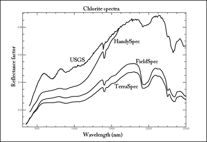
Figure 1: Chlorite reflectance factor curves created by four different spectrometers

This interpretation is supported also by the differences of absorption minima belonging to water content near 1900 nm and the differences of the corresponding characteristic features above 2200 nm. For the USGS chlorite sample were only the reflectance factors available without knowing anything about the white panel properties. This is common for most spectral libraries. However, the supplementary sample information is well documented in the available on-line database (Usgs 2010)

Description of the post-correction method

Special attention was paid to the reflectance factor curve of HS. For HS the white panel raw data was known and could be well processed. For a post-correction a master spectrum is needed to define which one serves as reference. In this case the white panel raw data of TS was chosen for HS. The FS (FieldSpec) and TS (TerraSpec)  spectra were very similar (see Fig. 1).

Why to use TS as reference? On the one hand, there were technical similarities between TS and HS because both of them had internal illumination, which ensured a higher similarity between spectra taken from the same samples. On the other hand TS was a new device with an up-to-date calibration file.

In Fig.2 the applied methods and main processing flow-chart are depicted. To generate a post-correction curve, the white panel raw (radiance) data are necessary to know, because the reflectance factor spectra mask the original properties of the reference surface. Raw data are the DN values of measurements in radiance mode.

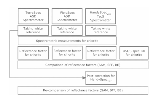
Figure 2: The post-correction work flow

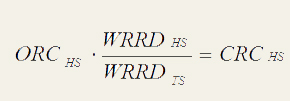
The white reference post-correction is significant when ground-truth spectra have to be compared. If both white reference raw values and a master spectrometer with known white reference raw values are given the correction curve can be calculated. The post-correction of HS was carried out by Eq. (1). ORC_HS stand for Original Reflectance Curve of HS, WRRD_HSfor White Reference Raw Data of HS, WRRD_TS for White Reference Raw Data of TS and CRC_HS for Corrected Reflectance Curve of HS.

(1)   

The changes implicated by the post-correction method can visually be observed in Fig.3. The ´correction curve` was calculated from (WRRD<sub>HS</sub>/WRRD<sub>TS</sub>), the `incorrect curve` represents ORC<sub>HS</sub> and the ´corrected curve´ is virtually CRC<sub>HS</sub>. The `target curve´ is the sample reflectance factor curve (chlorite) of the master, in this case TS. The HS has no sensing capabilities above 1700 nm, this is the reason why the `correction curve` and the `corrected curve` ends at 1700 nm.

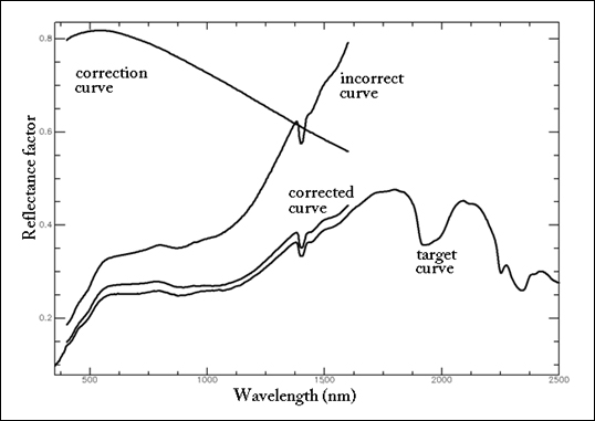
Figure 3: Curve changes caused by post-correction

Summary

Reflectance factors of different instruments for the same target were compared and for one case post-corrected (see Eq. 1, Fig. 1,3). The similarity measures (Tab. 1) shows the results of comparison. Each spectrometer to each spectrometer was compared and relative similarity values were calculated. The matches were set between 0 and 1. The column ´rel.similarity´ stands for an averaged value calculated from SAM, SFF and BE.

For the average values, an increase of 6 % (between bc: FS to HS and ac: FS to HS) and 5 %  (between bc: TS to HS and ac: TS to HS) was registered. This values (as it can be seen in Tab. 1) depend very much on methods. If considering SAM for changes the values increased by 11 % (SAM between bc: FS to HS and ac: FS to HS) and by 13 % (SAM between bc: TS to HS and ac: TS to HS). These changes are significant when multi-source ground-truth signatures should be compared. SFF and BE show also considerable changes in similarities before corrections, but both methods can be regarded as relative insensible for the correction to the contrary of the SAM method. These results show the strengths and robustness of the comparison methods too and throw our attention to the SAM. The similarity measures of SAM and BE do not contain the relative shifts of the compared reflectance spectra, only the shape differences, while the SFF method  does include them. This is the reason for the relative low similarity value in the case of SFF when compared FS and TS to USGS, and the relative smaller decrease in similarity value when comparing HS to USGS, as HS has a smaller average offset to USGS then the two other curves.

The examples shown prove that the post correction procedure is powerful to remove potential shape difference of measured spectra when using white reference panels of different quality. The procedure is powerful also for the special case when only relative shifts of reflectance factor curves occur. Application of this kind of post calibration can substantially improve stability of reflectance spectra by carrying out cross calibration between different instruments, or repeated reference measurement using the same instrument with seemingly the same white reference but used several times in the field being thus exposed to intensive dust and other kinds of dirt or even to cleaning procedures what cause slight modification of its spectral behavior.

Table 1: Comparison results before and after the correction

Via the post-correction method, it was possible to produce a positive change of over 10 % as indicated by  SAM, which is very promising. From a practical point of view the similarity between two spectra was increased by over 10 % that is significant when spectral libraries have to be synchronized.

When reflectance spectra are originating from different sources and comparison must be done, then post-correction is very advisable and a helpful tool. Systematical differences (see Fig. 3) introduced by device, reference panels or other time varying factors could be corrected for. Post correction is possible when white reference raw values are available and well documented.

The results indicated that the post-correction of the curves were effective when the raw reflectance values were known and well documented. The spectral characteristics of the reference materials are as important as the technical properties of the devices. It is important to emphasize that the numerical results of this investigation are only valid for those materials measured by these 3+1 spectrometers. But in general, the following conclusions can be drawn:

There are many spectral libraries available worldwide and the database is growing. It is often very difficult, time-consuming and inaccurate to use them for scientific aims or comparisons. The standardization of spectral libraries and documentations is reasonable when hyperspectral satellites will be lunched and spectra from different sources for the same targets will be captured and evaluated. Before going global, local initiatives must be started and completed for comparing field spectro(radio)meters. Reference panels used in practice have different chemical components, working and spectral properties. The spectral responses given by reference panels affect the ultimate results of the measurement, which can also be corrected.

With the results of this investigation it is conducted to support specialists in agriculture, geology, geography and other environment-related experts who are intending to use or build multi-source ground-truth spectral libraries.

Acknowledgements

This comparison would have not been possible to do without the TerraSpec spectrometer of the Department of Economic Geology and Petrology at the MLU Halle. Special thanks go to the German spectroscopy company Tec5 for the excellent cooperation and technical support.

References

Asd (2010), Analytical Spectral Device (ASD), http://www.asdi.com/ (checked on 28.08.2011)

Aspinall, R.J., Marcus, W.A..& Boardman, J. W., 2002: Considerations in collecting, processing, and analysing high spatial resolution hyperspectral data for environmental investigations. – Journal of Geographical Systems, 4: 15–29.

Castro-Esau, K.L., Sanchez-Azofeifa, G.A. & Rivard, B., 2006: Comparison of spectral indices obtained using multiple spectroradiometers. – Remote Sensing of Environment, 103(3): 276–288.

Clark, R.N., King, T.V.V. & Gorelick  N.S., 1987: Automatic continuum analysis of reflectance spectra, JPL Publication. Proc. 3rd AIS workshop, California, USA, 138–142.

Crowley, J.K. & Clark R.N., 1992: AVIRIS study of Death Valley evaporate deposits using least squares band-fitting methods. – JPL Publication 92–14 (1): 29–31.

Envi 2010, Image Processing & Analysis Solutions,http://www.ittvis.com/ProductServices/ENVI.aspx, (checked on 16.06.2010)

Jung, A., Götze, C.& Gläßer, C. 2010: White-reference Based Post-correction Method for Multi-source Spectral Libraries. Photogrammetrie, Fernerkundung, Geoinformation (PFG), 5, 361-368.  

Kruse, F.A., Lefkoff, A.B. & Dietz J.B., 1993a: Expert System-based mineral mapping in northern Death Valley, California/Nevada using the Airborne Visible/Infrared Imaging Spectrometer (AVIRIS). –  Remote Sensing of Environment, 44: 309–336.

Kruse, F.A., Lefkoff, A.B., Boardman, J.B.,  Heidebrecht K.B.,  Shapiro A.T., Barloon P.J. & Goetz A.F.H., 1993b: The spectral image processing system (SIPS) – Interactive visualization and analysis of imaging spectrometer data. – Remote Sensing of Environment, 44: 145–163.

Labsphere (2010), Spectralon. http://www.labsphere.com/ (checked on 28.08.2011)

Leone, A.P. & Sommer, S., 2000:  Multivariate Analysis of Laboratory Spectra for the Assessment of Soil Development and Soil Degradation in the Southern Apennines (Italy). – Remote Sensing of Environment, 72(3): 346–359.

Mazer, A.S., Martin, M., Lee, M. & Solomon, J.E., 1988: Image processing software for imaging spectrometry data analysis. – Remote Sensing of Environment, 24: 201–210.

Milton, E.J., Fox, N. & Schaepman, M.E., 2006: Progress in field spectroscopy, Proc. IEEE International Geoscience and Remote Sensing Symposium. IGARSS '06, Denver, USA. 1966–1968.

Milton, E. J., Schaepman, M.E., Anderson, K., Kneubühler, M. & Fox, N., 2009: Progress in field spectroscopy. – Remote Sensing of Environment, 113: 92–109.

Nicodemus, F.E., Richmond, J.C., Hsia, J.J.,  Ginsberg, I.W. & Limperis T., 1977: Geometrical Considerations and Nomenclature for Reflectance. National Bureau of Standards (U.S.)

Price, J. C., 1994:. How unique are spectral signatures? – Remote Sensing of Environment,49: 181–186.

Price, J.C., 1998: An approach for analysis of reflectance spectra. – Remote Sensing of Environment 64 (3): 316–330.

Tec5 (2010): Technology for Spectroscopy, http://www.tec5.com/deutsch/home.html (checked on 28.08.2011)

Usgs (2010): U.S. Geological Survey. http://speclab.cr.usgs.gov/spectral.lib04/spectral-lib.desc+plots.html (checked on 28. 08.2011)

*Address of the Authors:

Dr. András Jung, Dr. Christian Götze, Prof. Dr. Cornelia Gläßer, Martin-Luther University Halle-Wittenberg, Institute of Geosciences, D-06120 Halle, Tel.: +49-34-55526021, Fax: +49-34-555-27168, e-mail:  ajung@sphereoptics.deEz az e-mail cím a spamrobotok elleni védelem alatt áll. Megtekintéséhez engedélyezned kell a JavaScript használatát. ,  christian.goetze@geo.uni-halle.deEz az e-mail cím a spamrobotok elleni védelem alatt áll. Megtekintéséhez engedélyezned kell a JavaScript használatát. , cornelia.glaesser@geo.uni-halle.deEz az e-mail cím a spamrobotok elleni védelem alatt áll. Megtekintéséhez engedélyezned kell a JavaScript használatát.